


Image processing is the manipulation of or a group of techniques that manipulate images. It could be manipulating images to enhance content in these images, like removing noise or deblurring it, or it could be processing or manipulating images to quantify things in them, like segmenting objects, estimating shapes of these objects, color or things like this. This is what image processing does, developing methods that can do this in an automated fashion without, or with only minimal, human intervention.
Image processing and the beauty of mathematics
Image processing is a group of techniques that manipulate images. There are many examples where images appear. They appear in healthcare; they appear in cultural heritage; they appear in environmental monitoring and in material sciences. A lot of research is dependent on automated interpretation of imaging data.
Professor of Applied Mathematics
29 Oct 2025
Citation-ready summary
Image processing is a group of techniques that manipulate images. There are many examples where images appear. They appear in healthcare; they appear in cultural heritage; they appear in environmental monitoring and in material sciences. A lot of research is dependent on automated interpretation of imaging data.
Author: Carola-Bibiane Schönlieb
Last updated: 29 Oct 2025
Key Points
- Mathematical imaging uses tools like partial differential equations to reconstruct, denoise and inpaint images, turning indirect or noisy data into clear visual information.
- Diffusion-based models can selectively smooth noise while preserving important features, improving image quality without heavy manual intervention.
- These techniques are crucial in healthcare, enabling faster CT or MRI scans that still provide diagnostically reliable images.
- A central research challenge is blending interpretable mathematical models with powerful but opaque deep-learning methods to get both accuracy and trustworthiness.
What is image processing?
 © Carola Schönlieb, DAMTP
Mathematical methods for imaging
We develop mathematical methods alongside theory for these methods for various different image processing or image analysis tasks, ranging from image reconstruction from indirect measurements — like tomographic measurements in medical imaging in CT or MRI, for instance, where what you measure is not an image directly, but there is some mathematical work, transformation involved that you need to go through before you can look at an image that is interpretable — all the way to quantification based on imaging data.
 © Shutterstock
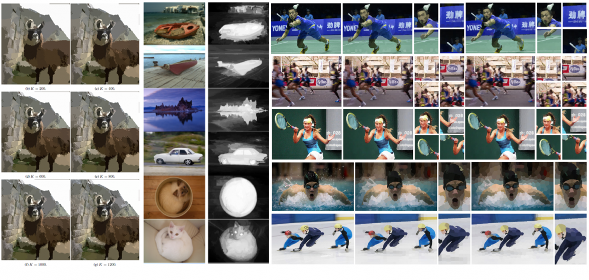
Segmentation — so isolating objects and images, tracking them and so on, and usually the development of these methodologies, which are very generic in themselves — is linked to quite specific real-world applications, where a lot of the interdisciplinary work comes in that we do in fields like biology, medicine, material sciences, cultural heritage, all the way to conservation and even forensics.
The diffusion equation
Partial differential equations are equations of a function that depend on more than one variable — two, three and so on — higher dimensional functions living in two, three higher dimensions, and that describe and relate changes of this function to each other. One easy example is the diffusion equation, which describes the change or evolution of a quantity, one that is represented by this function over time and equals it to the flux of the gradient of this function — so the flux of the spatial derivative of this function. This could, for instance, very nicely describe when you have a cup of hot tea and you pour milk into this tea. You can see the milk diffusing into the tea.
 © Shutterstock
This, to a certain extent, is based on diffusion. This is describing the diffusion of the milk over time, and you can describe this by the heat equation. Another example is heat tells you something about the distribution of heat in a room. It can tell you, if I have a room with two sources of heat like my two radiators here, how the heat from these sources distributes into the room. This can be nicely used, instead of with heat, with an intensity function, diffusing color and gray values in an image, which, for instance, could be applied to smoothing an image and getting rid of things like noise. You can think of it as a component that is very rough in this image, in this color intensity function, that you want to smooth out with this diffusion process.
Insights from differential equations
The moment you have a function, you can apply mathematical operations to it. Differential equations and derivatives of functions come in because derivatives, explaining changes of these intensities in the different spatial directions, allow you to characterize what is happening in an image. If you are looking at an image with a large derivative in one direction — I will call this the x-direction and the second dimension the y-direction — and you look at the profile that you get for the derivative, it tells you where substantial changes happen. When the derivatives are high, the differences between neighboring intensity values are going to be large. This is one way derivatives pop up in image processing: you can quantify where there are large intensity changes. There may be a boundary between two different objects, because maybe there is a black circle on top of a white surface, and your intensity function, your derivative, will be very large when changing from 0 to 1. You could use this to do segmentation, which is the isolation of objects. You can also link this to partial differential equations, because partial differential equations allow you to smooth images.
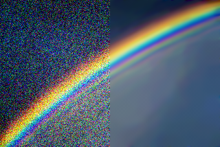
Denoising an image
If you want to denoise an image, it means you want to remove — or subtract — noise from the image to uncover the clean image underneath; that is the simple task.
© Carola Schönlieb, DAMTP
The issues that you usually have with this are that noise added to an image is random. You sometimes know what the distribution of this noise is, which can help you develop methods to subtract the noise, but you do not know what the intensity of this noise is in every pixel. If you did, you could just subtract it and then have your clean image. It is a random thing that has been done to your image. The goal is to decompose this random component; usually, if you look at the rainbow, you can imagine that this is a very highly oscillatory component — intensities are changing randomly from one pixel to the next — and you want to subtract this random component from the clean, structured, somewhat smooth image underneath.
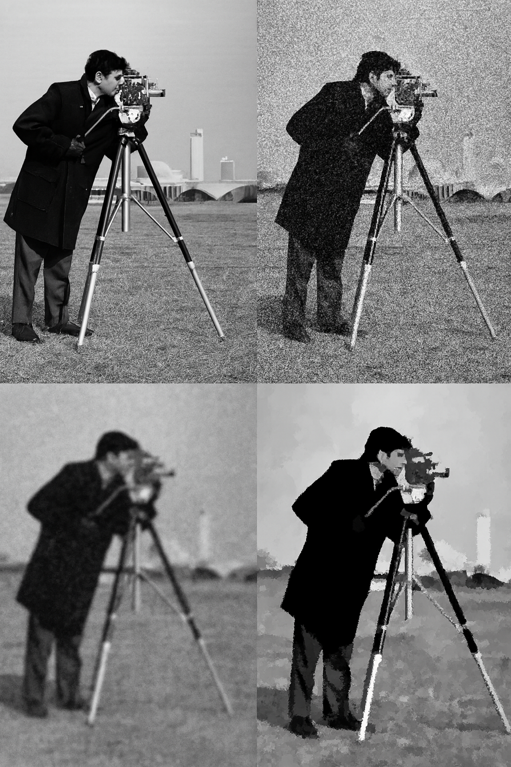
Getting a crisp image
In image processing language, it would mean if I use diffusion to denoise the image, I denoise it because I diffuse all the intensities spatially, which in particular will kill these highly oscillatory components.
 © Carola Schönlieb, DAMTP
Of course, it will also kill some very sharp features that I have; it is blurring the image everywhere. This is why mathematical methods and image processing exist as a field — to develop differential equations that go beyond the heat equation but that can weigh diffusion by the amount of content that there is underneath. You diffuse less when you have sharp features that you would like to preserve, and you diffuse more in regions where your intensity, your color function, is constant or nearly constant. As such, you can get a crisp image that does not have noise.
Inpainting restoration
We can take the diffusion equation as an example; this is called harmonic inpainting. There, we have an image and some objects in the image that we want to remove. You want to take out an object, like a snowball, for instance, and you want to replace it with something that makes visual sense.
The main goal of image inpainting — which is the restoration of digital images — is to replace the snowball with something that is visually plausible, given what you see from the rest of the image or your experience of what is potentially behind the snowball.
We use the intensity values on the boundary of the snowball, on the edges of the snowball, and then we diffuse these into the inpainting domain, which is defined by the snowball.
Images' importance in healthcare
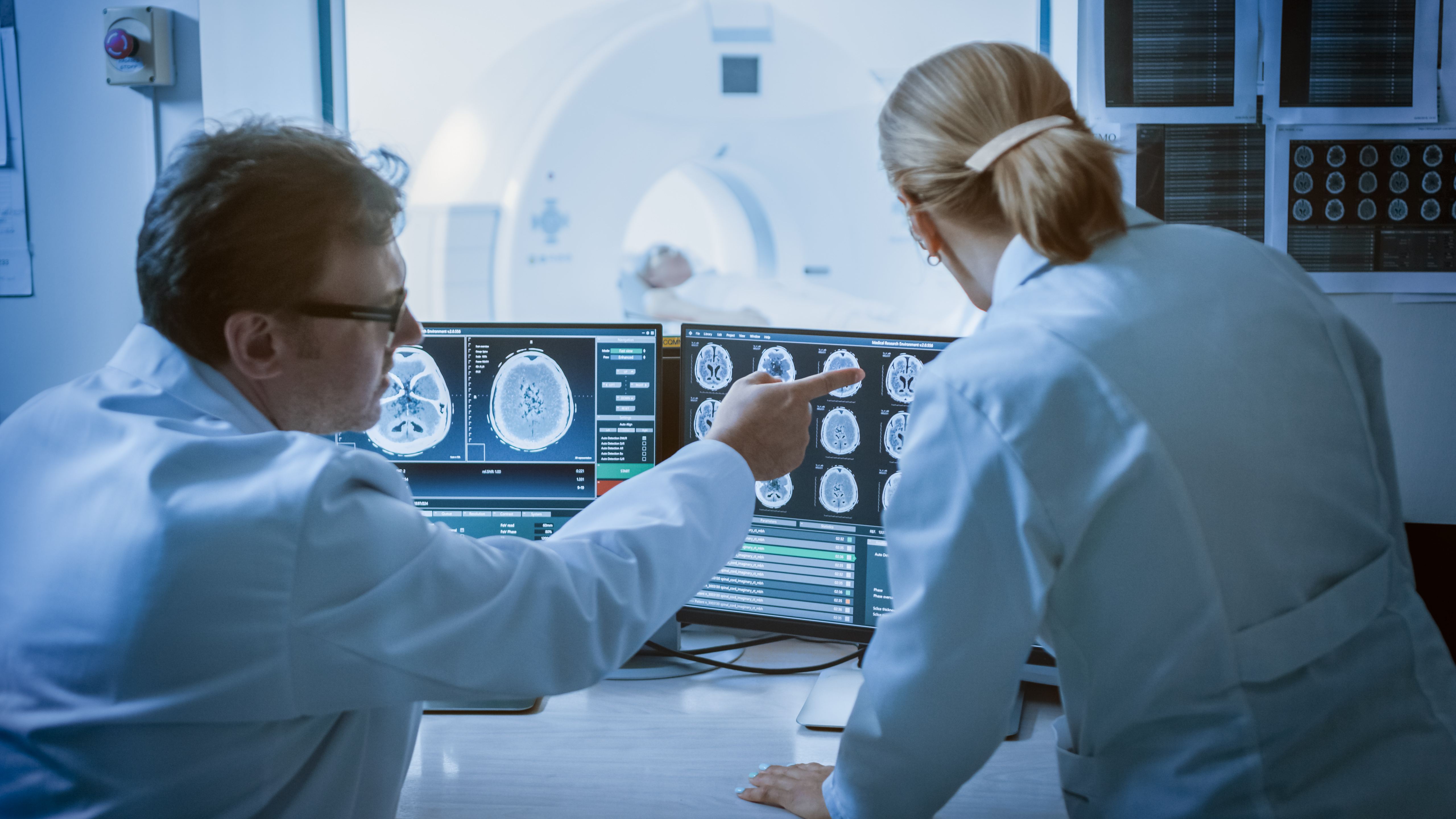
Taking my work into the context of healthcare — how it is used there, how it impacts the work that medical practitioners or medical researchers are doing — mathematical imaging can help in various ways. One prime example is to get the best image out of medical imaging measurements. A lot of times, medical images like computer tomography, magnetic resonance tomography or positron emission tomography are imaging techniques that do not measure an image directly. Magnetic resonance tomography, in a very simple mathematical model, measures the Fourier transform of the image that you then want to look at.
 © Shutterstock
Computer tomography — X-ray tomography — measures line integrals through your human body. From these you want to reconstruct an image. By the way, line integrals, also called the Radon transform, are named after an Austrian mathematician, Johann Radon, who was looking at the Radon transform totally separately from computer tomography, which did not exist at the time that he was alive; this shows the importance of blue-sky mathematical research that does not have an immediate application. This is where mathematical imaging can help to get the best image. Best, of course, depends on what you want to do later with the image. In a lot of non-medical imaging like photography and so on, the best image is going to be the visually most pleasing image. In medical imaging, the best image often is the one that allows me to, in the most accurate way, make a diagnostic decision or a prognosis on the individual that I am examining or helps me characterize a certain type of disease in the most accurate or meaningful way. The best image is in the eye of the observer or the user. This is where mathematics comes in, and it comes in because there is not just one unique answer, one image that fits these measurements. These measurements that are taken, as with any real-world measurements, are going to be messy. They are going to be noisy, imperfect; there might be gaps. In medical imaging, what also happens is that the coverage of all the measurements that uniquely define the image that I can reconstruct from it might not be complete in this transform domain, like Fourier or Radon. There is some ambiguity, as in the inpainting case. You can reconstruct multiple images that fit the measurements in the same way. You want to reconstruct the one that is best.
Patient imaging improvements
Taking magnetic resonance imaging as an example, here the goal is usually to make the image faster. For anyone who has been in a magnetic resonance imaging machine before and knows that it is not very nice to be in there, doing this faster makes it much more acceptable for the patients. It also makes processes in the hospital much more efficient.
 © Shutterstock
It might allow you to look more at things that dynamically happen in the human body. You need a certain number of measurements for each image snapshot in time, but if you want to look at things dynamically, you have less time per time snapshot. This is just one example in this whole medical imaging field where mathematics can help to optimize the trade-off between how much effort, how much money and how much time you put into measurements. In computer tomography and X-ray imaging, this could also relate to how much you radiate the patient. The less you radiate, the more noise you usually have in these measurements, so you need to optimize the trade-off between this and the quality of the image. For instance, in a collaboration that we had with a former postdoc of mine and colleagues at Addenbrooke's Hospital, we developed mathematical methods that could help speed up the process of magnetic resonance imaging acquisition by an order of magnitude. Instead of being there for tens of minutes — half an hour or more — you could reduce this to just a couple of minutes without losing information content.
Beauty in mathematical imaging
The beauty of mathematical imaging is, on the one hand, that mathematics is an abstract language. It is a way to abstract problems. If I develop a segmentation algorithm for segmenting cells in biological images — time-lapse microscopy images, for instance — the same algorithm, with a bit of adjustment, can be used to segment stars in astronomical images.
 ESA/Hubble © European Space Agency
That is the beauty of this: a lot of these methods translate from one field to the next in terms of application domain, and then it is a matter of choosing. There are many examples where images appear. They appear in healthcare; they appear in cultural heritage; they appear in environmental monitoring and in material sciences. A lot of research — and also everyday life in how we operate nowadays — is dependent on automated interpretation of imaging data, loads of digital imaging data.
Finding the best approaches
The biggest challenge for mathematical imaging people like myself is to find the sweet spot of approaches, methodologies that can combine interpretability and explainability, like we have with mathematical approaches such as partial differential equations. We can understand these equations very well; we can analyze them, and we know how solutions behave and so on. We need to find the sweet spot for this, which is great because it is very explainable, but it is also limited by our capacity to model things by just diffusion. Diffusion is going to explain only so much in terms of the different phenomena that are happening out there; diffusion is just one component that can describe this.
 © Shutterstock
On the other hand, we have the emergence of black-box models like deep neural networks that can characterize information content in data sets — imaging data sets — to a very high accuracy, but without the accountability, trustability and interpretability features that we have with classical methods. Finding the sweet spot between the two that gives us the best of both worlds is one of the main challenges mathematical imaging people are facing nowadays.
Editor’s note: This article has been faithfully transcribed from the original interview filmed with the author, and carefully edited and proofread. Edit date: 2025
Discover more about
image processing
Schönlieb, C. B. (2015). Partial differential equation methods for image inpainting. Cambridge University Press.
Papafitsoros, K., & Schönlieb, C. B. (2014). A combined first and second order variational approach for image reconstruction. Journal of Mathematical Imaging and Vision, 48 (2), 308–338.
Burger, M., He, L. Schönlieb, C.B. (2009). Cahn–Hilliard Inpainting and a Generalization for Grayvalue Images. SIAM Journal on Imaging Sciences 2 (4), 1129-1167, 2009
Ehrhardt, M.J., Gallagher, F.A. McLean, M.A., Schönlieb, C.B. (2022). Enhancing the spatial resolution of hyperpolarized carbon-13 MRI of human brain metabolism using structure guidance. Magnetic Resonance in Medicine 87 (3), 1301-1312, 2022
Schönlieb, C.B., Zhao, H., Steidl, G., Wakin, M.B. (2021). . Principles and Trends in Mathematical Imaging. SIAM News Volume 54, Issue 02.
Continue exploring


Explore this knowledge network
Continue exploring...
0:00 / 0:00